<?xml version="1.0" encoding="utf-8"?><feed xmlns="http://www.w3.org/2005/Atom" ><generator uri="https://jekyllrb.com/" version="3.10.0">Jekyll</generator><link href="https://arsalan-zafar.github.io/feed.xml" rel="self" type="application/atom+xml" /><link href="https://arsalan-zafar.github.io/" rel="alternate" type="text/html" /><updated>2026-05-05T19:48:35+00:00</updated><id>https://arsalan-zafar.github.io/feed.xml</id><title type="html">Arsalan Zafar</title><subtitle>personal description</subtitle><author><name>Arsalan Zafar</name><email>arsalanzafar@outlook.com</email></author><entry><title type="html">What We Have Built At Deep Render (So Far)</title><link href="https://arsalan-zafar.github.io/posts/2025/05/what-we-have-built-so-far/" rel="alternate" type="text/html" title="What We Have Built At Deep Render (So Far)" /><published>2025-05-22T00:00:00+00:00</published><updated>2025-05-22T00:00:00+00:00</updated><id>https://arsalan-zafar.github.io/posts/2025/05/What-We&apos;ve-Built-(So-Far)</id><content type="html" xml:base="https://arsalan-zafar.github.io/posts/2025/05/what-we-have-built-so-far/"><![CDATA[<p>Deep Render was built from the <a href="https://arsalan-zafar.github.io/posts/2024/04/solving-ai-based-compression/">ground up</a> to develop a production ready codec. We focused on developing an AI codec with low computational complexity and high compression efficiency. We worked with a relentless product focus, efficient tooling and process driven research. After 4 years in the trenches, we have developed a codec that can achieve real-time encode and decode with over 45% BD rate saving w.r.t. SVT-AV1. In other words, the world’s first AI codec.</p>

<p>To demonstrate what we’ve built so far, we’ve made our visual comparison app (<a href="https://eval.deeprender.ai">eval.deeprender.ai</a>) public - so everyone can assess our visual quality. We’ve also recently had <a href="https://www.linkedin.com/in/jan-ozer/">Jan Ozer</a> (streaming media) and <a href="https://fub.academia.edu/VittorioBaroncini/CurriculumVitae">Vittorio Baroncini</a> (ITU and MPEG testing chair) test our <a href="https://streaminglearningcenter.com/codecs/deep-render-an-ai-codec-that-encodes-in-ffmpeg-plays-in-vlc-and-outperforms-svt-av1.html">codec and compression performance claims</a>. In this blog, I’ll highlight our key achievements to date and touch on what we’re working towards now.</p>

<h1 id="compression-efficiency">Compression efficiency</h1>

<h2 id="subjective-metrics">Subjective metrics</h2>

<p>Our primary focus for compression efficiency is with respect to visual quality, the gold standard for evaluating quality in the compression industry. At Deep Render, we have a department dedicated to AI-based explicit and implicit density estimation, which allows us to leverage methods like diffusion models and GANs to enhance visual quality.</p>

<p>Verifying visual quality can be difficult, tedious and expensive. We have to pick between numerous methods that define how to structure visual studies, decide how to standardise viewing conditions, settle on a distribution strategy, crowdsource the results and finally, draw meaningful conclusions from the collected data in a format that is comprehensible. At Deep Render, we use three methods depending on the use case:</p>

<ul>
  <li><strong>Internal subjective evaluations</strong>: We use an application to distribute clips within Deep Render to collect votes.</li>
  <li><strong>Remotely crowdsourced votes through <a href="https://subjectify.us">Subjectify.us</a></strong>: We use Subjectify to distribute clips through the internet to thousands of participants and produce <a href="https://www.researchgate.net/publication/340060891_BSQ-rate_a_new_approach_for_video-codec_performance_comparison_and_drawbacks_of_current_solutions">BSQ rate plots</a>.</li>
  <li><strong>In-person standardized professional lab evaluations</strong>: We use a professional lab, such as Vittorio Baroncini VABTech lab to perform in-person standard p.910 DSIS ITU-T evaluations and retrieve BD-rates. This method is also used by the standard bodies when developing the ITU/MPEG codecs.</li>
</ul>

<p>To demonstrate our compression performance rigorously, we recently had an <a href="https://drive.google.com/file/d/1eU3gsBxfEFowRzxVYGcrsGK8BxgJLOe3/view">evaluation report</a> produced by Vittorio Baroncini, ITU/MPEG testing chair, using the P.910 DSIS method. These evaluations were performed in a professional laboratory setting with expert and naive viewers under the P.910 protocol. The results show that Deep Render achieves a ~45% bitrate reduction over SVT-AV1. Additionally, Jan Ozer published an evaluation of our subjective quality <a href="https://streaminglearningcenter.com/codecs/deep-render-an-ai-codec-that-encodes-in-ffmpeg-plays-in-vlc-and-outperforms-svt-av1.html">here</a> and reached a similar conclusion, demonstrating the visual quality gain in <a href="https://www.youtube.com/watch?v=D49ckpIoXB8&amp;t=2s&amp;ab_channel=JanOzer">this</a> video.</p>

<p>We believe this gain in visual quality is a significant result for the compression industry. It demonstrates that AI is the right tool to build the future of compression, and that future is here.</p>

<h2 id="objective-metrics">Objective metrics</h2>

<p>Deep Render as an organisation does not focus on objective metrics, but we still share them for academic purposes. Generally, we’ve found traditional metrics (PSNR/VMAF/SSIM) to not fully capture the subjective gains provided by AI codecs. Nonetheless, our traditional metrics are generally on par in BD-rate with SVT-AV1, all other things being equal. Jan Ozer evaluated and published these results <a href="https://streaminglearningcenter.com/codecs/deep-render-an-ai-codec-that-encodes-in-ffmpeg-plays-in-vlc-and-outperforms-svt-av1.html">here</a>. We think this is still a significant result as it demonstrates that even after ignoring the subjective improvements, AI codecs are already on par with traditional codecs while providing significant improvements in encoding complexity, roll-out speed and rate of progress.</p>

<h2 id="future-work">Future work</h2>

<p>Our codec currently operates in low-delay, p-frame only mode. We are actively working on building random access features such as hierarchical mini GOPs and B-frames. Excitingly, these models already provide a 10% BD rate improvement over SVT-AV1 in RA mode, and we expect to be outperforming traditional codecs by 40-50% on subjective metrics by the end of the year.</p>

<p>In addition to random access features, we’re also working on adding presets and additional rate control modes to our codec. These will enable encoding houses to trade complexity and coding efficiency based on their use cases.</p>

<h1 id="computational-complexity">Computational complexity</h1>

<p>A key critique of AI codecs is their inability to encode and decode without expensive GPUs. This is true for AI compression modes in academia, such as<a href="https://github.com/microsoft/DCVC">DCVC</a> series from Microsoft, however, as demonstrated by Jan’s testing, Deep Render’s AI codec can seamlessly and efficiently encode and decode on everyday, widely available hardware while providing 45% BD rate gains. Without a doubt, this has been a key achievement of our team. Without this capability, AI codecs remain a mythical technology only future generations will unlock.</p>

<h2 id="encode--decode">Encode &amp; Decode</h2>

<p>When encoding and decoding on Apple M series chips, our codec was able to achieve 22 and 70+ respectively as verified by Jan Ozer <a href="https://www.youtube.com/watch?v=D49ckpIoXB8&amp;t=2s&amp;ab_channel=JanOzer">here</a>. Internally, we have models that can hit 30+ and 100+ fps on encode and decode respectively which will go into production later this year. These internal models have benefited from research breakthroughs in the past two months, unlocking significant computational efficiency gains. Achieving a decode speed of 100 FPS on widely available hardware while providing a 45% BD-rate gain over AV1 demonstrates that AI is the right tool for compression and AI codecs are imminently ready to dominate the codec industry, with Deep Render leading the charge.</p>

<h2 id="bdt-battery-drain-time">BDT (Battery drain time)</h2>

<p>Besides encode and decode speed, the concept of battery drain time is important for a production ready codec. Battery drain time is defined as the time taken to drain the battery from 100% to 0% on a given device while playing back a sequence. On phones from the last three years, our next production model will be able to achieve up to 15 hours of BDT, while the dav1d decoder is able to achieve around 16-18 hours, all other things being equal. Even though the dav1d decoder currently beats out Deep Render, we don’t see this as an issue since we’re seeing an impressive and consistent reduction in computational complexity every quarter. We also believe that a BDT of 15 hours on phones is above the threshold for widespread deployment.</p>

<h2 id="future-work-1">Future work</h2>

<p>While we think a BDT of 15 hours is sufficient for significant deployment, we are confident we can increase this to 18-20 hours through methods such as content-adaptive encoding paths. We believe this can be achieved by early next year and will enable us to deploy AI codecs to an even wider audience by targeting lower-end and older devices.</p>

<h1 id="device-reach">Device reach</h1>

<p>A key attraction of the Deep Render codec is that it does not require specialised hardware to decode. Deep Render uses widely available commodity hardware like the NPU available on Apple, Qualcomm, MediaTek and many other devices. This has two significant advantages.</p>

<p>Firstly, Deep Render is decoupled from the custom hardware development and adoption cycles as it does not require them for efficient encoding and decoding. Already, there are billions of devices that can encode and decode our AI codec efficiently. What’s even more exciting is the rate at which the capability of these NPUs is improving. In the last four years, Apple NPUs have gone from 11 TOPs to 35 TOPs, Qualcomm NPUs from 26 to 50 TOPs and Intel NPUs will be going from 11 TOPs in Meteor Lake to 50+ in Lunar and Panther Lake chips. Deep Render can easily leverage this trend to further improve compression performance, BDT, and playback frame rates.</p>

<p>Secondly, since our codec is essentially a software codec, we can readily deploy improved codecs with a higher frequency as we unlock more gains through our ongoing research efforts. The current 45% BD rate gain over AV1 is just the start, and we expect our coding gains to continue to improve as we continue to explore the frontier of AI. On top of this, we can build techniques such as <a href="https://arsalan-zafar.github.io/posts/2025/03/future-of-ai-based-compression/">specialisation</a> into production systems to really enhance products and improve engagement.</p>

<p>The codec world is used to having a new codec every 10 years and dealing with a slow adoption curve as hardware lags behind. AI codecs remove these constraints entirely while providing significantly more gains, flexibility and a brighter future</p>

<h1 id="deployability">Deployability</h1>

<p>Having a codec without any deployment infrastructure hinders testing, roll-out and ultimately adoption. Deep Render’s Engineering team has been focused on building real world integrations. We’ve focused on making our AI codec easy to test, playback and deploy.</p>

<p>To allow seamless testing and deployment, we developed <a href="https://www.youtube.com/watch?v=Bk8iCrvZt5w&amp;ab_channel=JanOzer">FFmpeg binaries</a> and parallel production APIs. Encoded clips are containerised using MP4 containers, ideal for DASH streaming. To stream encoded clips, we support the generation of manifest files (e.g., MPD for DASH) that describe available video qualities, bitrates, segment locations and other metadata. Finally, for playback on edge devices, we support playback through VLC which can playback DASH.</p>

<p>While we think we’ve made significant progress in our integrations, we’re continuing to build out our APIs to enable deeper and wider integration into the compression ecosystem. This year, we’re adding a low-power mode to enable wider device reach, additional rate control modes, presets, and random access features.</p>

<h1 id="looking-ahead">Looking ahead</h1>

<p>Our team has made incredible progress in the last few years, and we fundamentally believe that AI is the right tool to build codecs, as demonstrated by our results. However, we’re just at the beginning of the AI codec development and progress arc. If we project ourselves 5 years into the future, without a doubt, the codec industry will be dominated by AI codecs with the following features:</p>

<ul>
  <li>There will be multiple proprietary AI codecs on the market, and encoding houses will own their own AI codec, reducing reliance on standard bodies</li>
  <li>There will be different codecs per use case, media type, film title and even person</li>
  <li>NPUs will be widespread and boast 100+ TOPs of compute, enabling efficient and seamless deployment</li>
  <li>AI codecs will be providing 3- 4x improvements over traditional codecs</li>
</ul>

<p>We think the world will benefit greatly from this future, and the Deep Render team will continue working toward this future.</p>

<hr />

<p><em>Special thanks to Allie, Clare, Chris and Sebastjan for the reviews.</em></p>]]></content><author><name>Arsalan Zafar</name><email>arsalanzafar@outlook.com</email></author><category term="AI based compression" /><category term="AI codecs" /><category term="video compression" /><summary type="html"><![CDATA[Deep Render was built from the ground up to develop a production ready codec. We focused on developing an AI codec with low computational complexity and high compression efficiency. We worked with a relentless product focus, efficient tooling and process driven research. After 4 years in the trenches, we have developed a codec that can achieve real-time encode and decode with over 45% BD rate saving w.r.t. SVT-AV1. In other words, the world’s first AI codec.]]></summary></entry><entry><title type="html">Future of AI based compression</title><link href="https://arsalan-zafar.github.io/posts/2025/03/future-of-ai-based-compression/" rel="alternate" type="text/html" title="Future of AI based compression" /><published>2025-03-17T00:00:00+00:00</published><updated>2025-03-17T00:00:00+00:00</updated><id>https://arsalan-zafar.github.io/posts/2025/03/Future-of-AI-Based-Compression</id><content type="html" xml:base="https://arsalan-zafar.github.io/posts/2025/03/future-of-ai-based-compression/"><![CDATA[<p>Deep Render recently introduced the first AI codec into FFmpeg and VLC. This marks a significant step for AI codecs, making them readily available in tools widely used in the compression industry. Deep Render will continue to push the frontier of AI codecs by further improving compression performance, providing support for more hardware platforms and improving feature diversity.</p>

<p>However, AI codecs hold far more promise and opportunities than the initial 40% compression efficiency gains they have already achieved. The one I’ll be highlighting in this blog is called specialisation.</p>

<h1 id="specialisation">Specialisation</h1>

<p>Since AI codecs are learnt from data, we can be creative with the data they’re learned from to affect change in the model’s behaviour. Specialisation is a method developed at Deep Render that limits the training data to a subset of all the data in the world. For example, it is possible to train an AI codec only on sequences of dogs. This makes the codec extremely good at compressing dogs and degrades performance elsewhere. This gives us a dog-specific codec, which would be great when compressing sequences of dogs. This is a contrived example, but this ability to control training data has some significant real-world applications. Specialisation can already provide a 30% efficiency gain, on top of the 40% gain that Deep Render’s codec already provides, leading to a total of ~50% compression efficiency gains.</p>

<h2 id="per-title-film-encoding">Per title film encoding</h2>

<p>To set the scene, film titles are encoded once and streamed tens to hundreds of millions of times. On a high level, the process works as follows: A film title is encoded, and the bitstream is stored on many local servers around the world. When a user wants to view this title, it’s fetched from a local server, decoded and displayed on the screen.</p>

<p>With AI codecs and their ability to specialise, we can train our SOTA (state-of-the-art) AI codec on this single title by limiting the training data to only sequences from this film title and realise an additional 30% compression efficiency gains, leading to a total of 50% bitrate reduction. Once this model is trained, we can use it to compress sequences and create bitstreams. The total model size is anywhere between 300KB to 2MB, which means it’s small enough to stream over the network. With this in mind, the new content delivery pipeline would look as follows: An AI codec is used to specialise on a film title, giving us a title-specific codec. This encode of this specialised model is used to create bitstreams. When a user wants to view this title, we first stream the specialised decoder and then the bitstreams. On the client end, we use the streamed decoder to decode the arriving bitstreams. This gives rise to per-title codecs, which are streamable and capable of realising an additional 30% on top of the already excellent compression efficiency provided by AI codecs. In this world, we would now have a codec per film title, but since there is a power law in the popularity of films, we can reap most of the benefits by applying this only for the top titles.</p>

<p>As an extension to this, we can also utilise the method described above on film chunks, as Netflix does with their dynamic optimiser, to achieve a per-chunk codec. This will unlock even more gains since we’re further restricting the data domain on which our model is trained. This, of course, has to be traded off with having to stream a codec per chunk, which could offset any savings.</p>

<h2 id="per-game-title-encoding">Per game title encoding</h2>

<p>Similar to the example above, we can also restrict the training data of an AI codec to gameplay from a specific game. This would result in per-title codecs for games; for example, we could have a codec specialised to Call of Duty used to encode Call of Duty gameplay and generate the respective bitstreams to be sent across the network.</p>

<p>For cloud gaming platforms, when a user requests to play a specific game, the platform would first stream the game-specific AI codec and then the bitstreams generated by this codec. This would significantly reduce the bits needed for cloud gaming by providing a 30% additional gain, leading to a total of 50% bitrate reduction.</p>

<p>Additionally, games often have visually distinct maps and regions. For example, you can select to play Call of Duty in different terrains, which essentially means the game loads and renders a certain set of textures. We can generate a codec per map or terrain, which allows us to specialise our codec even further, reaping further compression efficiency gains. You can extend this concept to any visually distinct regions of a game, such as different sections of a given game map.</p>

<h2 id="per-person-codec-for-video-conferencing">Per person codec for video conferencing</h2>

<p>We can also apply specialisation in video conferencing to achieve further bitrate reductions.</p>

<p>Imagine the following addition to your most popular video conferencing app. When you download and set up a video conferencing app, it asks you to record a 10 second clip of yourself repeating some sentences. This recorded clip is used to create an AI codec specialised to you, which enables high-quality and smooth video conferencing for you. Would users want this?</p>

<p>How can a video conferencing provider achieve these additional gains? They would take the 10 second clip and apply domain randomisation to create more data samples. Next, they would use this data to train an AI codec specialised to the person. Once this is complete, a video conferencing call will look as follows. At the start of a call, say a 1-1 call, each user would stream their personalised AI decoder to the other. They would then use their personalised AI encoders to encode their webcam stream and send the bitstream to the other user, who would decode it with the AI decoder specialised to the person who sent the bitstream.</p>

<p>This has the potential to significantly improve compression performance. Currently, Deep Render provides a 70% improvement over AV1 in talking heads, and a per-person specialised codec would add another 30%, leading to 5x improvement in video conferencing compared to AV1, a remarkable feat.</p>

<h1 id="looking-forward">Looking forward</h1>

<p>As evident from previous sections, due to the paradigm change, AI codecs and specialisation afford unbounded creativity and compression efficiency gains. To date, Deep Render has verified that specialisation can give up to 30% efficiency gains but we don’t know the limit. On the other hand, we have not implemented any of the above pipelines in production. Inevitably, there will be challenges when productionising, and some trade-offs will have to be made, but I think it will be worth it. I firmly believe that AI codecs are the future of compression and that specialised AI codecs are the future of AI codecs.</p>]]></content><author><name>Arsalan Zafar</name><email>arsalanzafar@outlook.com</email></author><category term="AI based compression" /><category term="AI codecs" /><category term="video compression" /><summary type="html"><![CDATA[Deep Render recently introduced the first AI codec into FFmpeg and VLC. This marks a significant step for AI codecs, making them readily available in tools widely used in the compression industry. Deep Render will continue to push the frontier of AI codecs by further improving compression performance, providing support for more hardware platforms and improving feature diversity.]]></summary></entry><entry><title type="html">Solving AI based compression</title><link href="https://arsalan-zafar.github.io/posts/2024/04/solving-ai-based-compression/" rel="alternate" type="text/html" title="Solving AI based compression" /><published>2024-04-08T00:00:00+00:00</published><updated>2024-04-08T00:00:00+00:00</updated><id>https://arsalan-zafar.github.io/posts/2024/04/Solving-AI-Based-Compression</id><content type="html" xml:base="https://arsalan-zafar.github.io/posts/2024/04/solving-ai-based-compression/"><![CDATA[<p>Deep Render recently shipped the world’s first AI codec to its customers. This result follows two years of careful research, gruelling engineering, and relentless product focus. I’ll take some time to share some thoughts on the research and engineering that went into solving AI-based compression.</p>

<h1 id="the-research">The research</h1>

<p>A key critique we have of the current AI-based compression field is their disregard for model complexity. The community has opted for improved compression performance through increased model size at the cost of production feasibility. At the extreme, you can argue that most gains made in AI-based compression over the last few years have simply been due to increasing model complexity. A symptom of this doctrine is the annual CLIC competition, which, to this day, lacks any target for model complexity.</p>

<p>Model complexity matters because it’s intricately linked with compression performance. If we want to see AI codecs in production in the short term, we must optimise compression performance per operation (model complexity). It will come as no surprise that this is our north star.</p>

<p>During the research phase for our codec, we jointly optimise compression performance and model complexity. We’ve developed systems that enable us to implement, train, and measure compression performance and model complexity within a few days. Given this streamlined workflow, we have diligently worked through major unsolved problems limiting AI-based compression: INT8 to float compression performance gap, temporal visual consistency, efficient edge device execution, and cross-platform consistency.</p>

<p>As a fun sidenote, AI-based codecs, if not trained correctly, can produce fascinating videos. Here’s an example:</p>

<h1 id="the-engineering">The engineering</h1>

<p>Productisation requires an immense amount of raw engineering. Historically, AI-based compression-esque companies have been heavily focused on research, demonstrated by the unimodal composition of their teams. A well-balanced team should be able to bridge innovations over the non-trivial gap between research and production, enabling the widespread adoption of exciting technologies. It will come as no surprise that Deep Render places an equal importance on engineering and research. We have teams that focus on ML engineering, Device integration and Infrastructure.</p>

<h2 id="ml-engineering">ML engineering</h2>

<p>Developing several independent and complex innovations during the research phase is only part of the puzzle. The final model must provide the joint benefits of these innovations. It falls on our ML Engineering team to organise innovations, perform integration and training to deliver production-ready checkpoints. They run between 200-500 integration experiments to achieve the final stable models for each iteration of our codec. Training schedules, datasets and learning rate length are all hyperparameters that are ablated in parallel, as they can significantly impact compression performance.</p>

<p>Once the final weights are ready, our evaluation team uses their extensive in-house benchmarking library to thoroughly benchmark our models against all traditional codecs, resulting in an array of objective and subjective metrics. As part of these evaluations, we partner with Subjectify to crowd-source subjective evaluations worldwide, resulting in over 10,000 votes per evaluation.</p>

<h2 id="device-integration">Device integration</h2>

<p>AI is a cloud-centric industry. The majority of the widely used AI applications run inference on the cloud. The simple reason for this is that executing well-performing methods efficiently on edge devices is challenging. To alleviate this, chip manufacturers are continually improving the hardware and software stack for edge AI. We’re seeing incredible inter-generation improvement in hardware capabilities. However, the APIs, the gateway to the hardware, are often rigid, poorly documented and bug-prone. This is to be expected, given where we are in the maturity cycle for AI.</p>

<p>AI-based compression is a field that does not have the luxury of being cloud-centric, as decodes have to be run on edge devices. As an antidote to the nascency of edge AI APIs, Deep Render has partnered with all major hardware providers to collaborate on their development. This has created a feedback loop between our implementation process and the vendor’s development process, greatly speeding up our development.</p>

<p>Deep Render follows the standard device porting logic. We produce JIT-traced models using TorchScript, which are consumed by vendor API converters to create modules capable of executing on edge devices. Deep Render often uses custom operators that are currently unsupported by vendor APIs. For these, we write highly optimised implementations in OpenCL or Metal. Once we have all modules on the device, we optimise memory movement, execution graph, operator selection, and parallelism using custom software developed at Deep Render. Finally, the optimised codec undergoes extensive testing using a framework set up by our infrastructure team, reporting back power consumption, frame rate and compression performance across various devices and sequences. Once the tests have passed, the codec is tagged for release.</p>

<h2 id="infrastructure">Infrastructure</h2>

<p>To support our engineering effort, we have an infrastructure team dedicated to maintaining code, testing, and hardware needs. Their primary aim is to create a pipeline that allows us to go from research code to results efficiently. They turn code into coding gains. Alongside optimising the software and testing infrastructure, they maintain our on-premise training systems, with over 150 compute nodes custom-built to solve compression.</p>

<h1 id="looking-forward">Looking forward</h1>

<p>Our fundamental belief is that AI is the tool that will allow humanity to reach the compression limit. Deep Render is spearheading this goal and is perfectly placed to make the most progress towards it. Our models have surpassed 45 years of incumbent research in two years, and we have internal research showing that we’ve barely scratched the surface. Who’s to say what the next two will bring?</p>]]></content><author><name>Arsalan Zafar</name><email>arsalanzafar@outlook.com</email></author><category term="AI based compression" /><category term="AI codecs" /><category term="video compression" /><summary type="html"><![CDATA[Deep Render recently shipped the world’s first AI codec to its customers. This result follows two years of careful research, gruelling engineering, and relentless product focus. I’ll take some time to share some thoughts on the research and engineering that went into solving AI-based compression.]]></summary></entry><entry><title type="html">Transformer and ViT dataflow notation</title><link href="https://arsalan-zafar.github.io/posts/2021/01/vit-transformation-notation/" rel="alternate" type="text/html" title="Transformer and ViT dataflow notation" /><published>2021-12-15T00:00:00+00:00</published><updated>2021-12-15T00:00:00+00:00</updated><id>https://arsalan-zafar.github.io/posts/2021/01/ViT-Transformation-Notation_up</id><content type="html" xml:base="https://arsalan-zafar.github.io/posts/2021/01/vit-transformation-notation/"><![CDATA[<p>When reviewing the transformer and ViT literature, to get an intuitive understanding of the various model layers and how the input tokens are manipulated, I found it helpful to map out the data flow through the model in matrix notation. I couldn’t find this anywhere so I thought I’d share it.</p>

<hr />

<h1 id="part-i-minigpt-foundation">Part I: miniGPT Foundation</h1>

<p>This section covers the matrix notation for miniGPT.</p>

<h2 id="notation--sizes-minigpt">Notation / sizes (miniGPT)</h2>

<ul>
  <li>Batch \(B\), sequence length \(T\), vocab size \(V\)</li>
  <li>Model width \(D\) (aka \(d_{\text{model}}\))</li>
  <li>MLP hidden width \(d_{\text{ff}}\) (often \(4D\))</li>
  <li>Single head so \(d_k=d_v=D\) (keeps shapes simple)</li>
  <li>Pre-LayerNorm residual layout (GPT-2/miniGPT style)</li>
</ul>

<hr />

<h2 id="0-inputs-embeddings-positions">0) Inputs, embeddings, positions</h2>

<ul>
  <li>Token indices: \(\mathbf{t}\in\{1,\dots,V\}^{B\times T}\)</li>
  <li>Token embedding matrix: \(E\in\mathbb{R}^{V\times D}\)</li>
  <li>Learned positional embeddings: \(P\in\mathbb{R}^{T\times D}\)</li>
</ul>

<p><strong>Lookup + add positions</strong>
\(X^{(0)} \;=\; E[\mathbf{t}] + P \quad\in\; \mathbb{R}^{B\times T\times D}\)</p>

<hr />

<h2 id="1-a-single-transformer-block-ell1dotsl">1) A single Transformer block \(\ell=1,\dots,L\)</h2>

<h3 id="11-pre-norm-attention">1.1 Pre-norm (attention)</h3>

<p>LayerNorm acts per token (last dim):
\(\tilde{X} \;=\; \mathrm{LN}^{(\ell)}_{\mathrm{attn}}\!\left(X^{(\ell-1)}\right) \;\in\; \mathbb{R}^{B\times T\times D}\)</p>

<p>(Each token vector \(x\in\mathbb{R}^{D}\) is normalized and then scaled/shifted by \(\gamma,\beta\in\mathbb{R}^{D}\).)</p>

<h3 id="12-single-head-qkv-projections">1.2 Single-head Q/K/V projections</h3>

<p>Weights \(W_Q^{(\ell)},W_K^{(\ell)},W_V^{(\ell)}\in\mathbb{R}^{D\times D}\):
\(Q \;=\; \tilde{X}W_Q^{(\ell)}, \qquad K \;=\; \tilde{X}W_K^{(\ell)}, \qquad V \;=\; \tilde{X}W_V^{(\ell)} \quad\in\; \mathbb{R}^{B\times T\times D}\)</p>

<h3 id="13-scaled-dot-product-attention-causal">1.3 Scaled dot-product attention (causal)</h3>

<p>Scores (pairwise dot products per batch):
\(S \;=\; \frac{QK^{\top}}{\sqrt{D}} \;+\; M \quad\in\; \mathbb{R}^{B\times T\times T}\)</p>

<p>where \(M_{ij}=0\) if \(j\le i\) and \(M_{ij}=-\infty\) if \(j&gt;i\) (upper-triangular causal mask).</p>

<p>Row-wise softmax:
\(A \;=\; \mathrm{softmax}(S) \;\in\; \mathbb{R}^{B\times T\times T}\)</p>

<p>Weighted sum of values:
\(H \;=\; A\,V \;\in\; \mathbb{R}^{B\times T\times D}\)</p>

<p>Output projection \(W_O^{(\ell)}\in\mathbb{R}^{D\times D}\):
\(O \;=\; H\,W_O^{(\ell)} \;\in\; \mathbb{R}^{B\times T\times D}\)</p>

<p>Residual add:
\(X' \;=\; X^{(\ell-1)} + O \;\in\; \mathbb{R}^{B\times T\times D}\)</p>

<h3 id="14-pre-norm-mlp">1.4 Pre-norm (MLP)</h3>

\[\hat{X} \;=\; \mathrm{LN}^{(\ell)}_{\mathrm{mlp}}(X') \;\in\; \mathbb{R}^{B\times T\times D}\]

<h3 id="15-mlp-with-gelu">1.5 MLP with GELU</h3>

<p>Weights \(W_1^{(\ell)}\in\mathbb{R}^{D\times d_{\text{ff}}}\), \(W_2^{(\ell)}\in\mathbb{R}^{d_{\text{ff}}\times D}\) (biases optional):
\(U \;=\; \hat{X}W_1^{(\ell)} + b_1^{(\ell)} \;\in\; \mathbb{R}^{B\times T\times d_{\text{ff}}}\)</p>

\[G \;=\; \mathrm{GELU}(U) \;\in\; \mathbb{R}^{B\times T\times d_{\text{ff}}}\]

\[M \;=\; G\,W_2^{(\ell)} + b_2^{(\ell)} \;\in\; \mathbb{R}^{B\times T\times D}\]

<p>Residual add:
\(X^{(\ell)} \;=\; X' + M \;\in\; \mathbb{R}^{B\times T\times D}\)</p>

<p>(Repeat this block for \(\ell=1,\dots,L\).)</p>

<hr />

<h2 id="2-output-head-rightarrow-logits">2) Output head \(\rightarrow\) logits</h2>

<p>Final LayerNorm:
\(X_f \;=\; \mathrm{LN}_f\!\left(X^{(L)}\right) \;\in\; \mathbb{R}^{B\times T\times D}\)</p>

<p>Linear head to vocab. Two common options:</p>

<p><strong>(a) Weight tying (GPT-style):</strong>
\(Z \;=\; X_f\,E^{\top} \;\in\; \mathbb{R}^{B\times T\times V}\)</p>

<p><strong>(b) Separate head:</strong>
\(Z \;=\; X_f\,W_{\text{vocab}} + b_{\text{vocab}}, \qquad W_{\text{vocab}}\in\mathbb{R}^{D\times V}\)</p>

<p>These logits \(Z\) give the next-token distribution via softmax over the vocab dimension; training uses cross-entropy with targets shifted by one.</p>

<hr />

<h2 id="summary">Summary</h2>

<ul>
  <li><strong>Embeddings:</strong> \(X^{(0)}=E[\mathbf{t}]+P \;\in\; [B,T,D]\)</li>
  <li><strong>Attn pre-LN:</strong> \(\tilde{X}=\mathrm{LN}(X^{(\ell-1)}) \;\in\; [B,T,D]\)</li>
  <li><strong>Q/K/V:</strong> \(Q=\tilde{X}W_Q,\; K=\tilde{X}W_K,\; V=\tilde{X}W_V \;\in\; [B,T,D]\)</li>
  <li><strong>Scores:</strong> \(S=QK^{\top}/\sqrt{D}+M \;\in\; [B,T,T]\)</li>
  <li><strong>Weights:</strong> \(A=\mathrm{softmax}(S) \;\in\; [B,T,T]\)</li>
  <li><strong>Context:</strong> \(H=A\,V \;\in\; [B,T,D]\)</li>
  <li><strong>Proj:</strong> \(O=H\,W_O \;\in\; [B,T,D]\)</li>
  <li><strong>Residual:</strong> \(X'=X^{(\ell-1)}+O \;\in\; [B,T,D]\)</li>
  <li><strong>MLP pre-LN:</strong> \(\hat{X}=\mathrm{LN}(X') \;\in\; [B,T,D]\)</li>
  <li><strong>MLP:</strong> \(G=\mathrm{GELU}(\hat{X}W_1+b_1) \;\in\; [B,T,d_{\text{ff}}]\)</li>
  <li><strong>MLP proj:</strong> \(M=G\,W_2+b_2 \;\in\; [B,T,D]\)</li>
  <li><strong>Residual:</strong> \(X^{(\ell)}=X'+M \;\in\; [B,T,D]\)</li>
  <li><strong>Final:</strong> \(X_f=\mathrm{LN}_f(X^{(L)}) \;\in\; [B,T,D]\)</li>
  <li><strong>Logits:</strong> \(Z=X_fE^{\top}\) (tied) <strong>or</strong> \(Z=X_fW_{\text{vocab}}\) (untied) \(\;\in\; [B,T,V]\)</li>
</ul>

<hr />

<h1 id="part-ii-vit--text-single-stream">Part II: ViT → Text (Single-Stream)</h1>

<p>Building on the miniGPT foundation, we can now extend to Vision Transformers that process both image and text data in a unified architecture. The primary difference is that we’d now like to take our image, patchify it and map that patches into tokens so we can have the text and image data in the same format and domain to be processed by our attention layers.</p>

<p>We also assume that we want text output.</p>

<h2 id="notation--sizes-vit-extension">Notation / sizes (ViT Extension)</h2>

<ul>
  <li>Batch \(B\); image \((H\times W)\) with channels \(C\)</li>
  <li>Patch size \(P\); number of patches \(N=\frac{H}{P}\cdot\frac{W}{P}\)</li>
  <li>Text length \(T\), vocab size \(V\)</li>
  <li>Model width \(D\), MLP hidden width \(d_{\text{ff}}\) (e.g., \(4D\))</li>
  <li>Single head so \(d_k=d_v=D\) (keeps shapes simple)</li>
  <li>Pre-LayerNorm residual layout (GPT-style)</li>
</ul>

<hr />

<h2 id="0-inputs--tokens">0) Inputs → tokens</h2>

<h3 id="01-image--patch-tokens">0.1 Image → patch tokens</h3>

<p>Define an <strong>unfold</strong> operator \(\mathcal{U}\) that extracts flattened non-overlapping patches:
\(\mathcal{U}:\ \mathbb{R}^{B\times C\times H\times W}\ \to\ \mathbb{R}^{B\times N\times (C P^2)}\)</p>

<p>Let the image batch be \(X_{\text{img}}\in\mathbb{R}^{B\times C\times H\times W}\). Then
\(X_{\text{patch}}=\mathcal{U}(X_{\text{img}})\ \in\ \mathbb{R}^{B\times N\times (C P^2)}\)</p>

<p>Linear patch projection (ViT style):
\(W_{\text{patch}}\in\mathbb{R}^{(C P^2)\times D},\quad b_{\text{patch}}\in\mathbb{R}^{D},\qquad I=X_{\text{patch}}\,W_{\text{patch}}+b_{\text{patch}}\ \in\ \mathbb{R}^{B\times N\times D}\)</p>

<p>(Equivalently: a Conv2d with kernel\(=\)stride\(=P\) giving \([B,D,H/P,W/P]\), then flatten to \([B,N,D]\).)</p>

<p>Add <strong>2D positional</strong> embeddings for image patches (flattened scan order):
\(P_{\text{img}}\in\mathbb{R}^{N\times D},\qquad I^{(0)}=I+P_{\text{img}}\ \in\ \mathbb{R}^{B\times N\times D}\)</p>

<p>(Optional <strong>type</strong>/modality embedding \(T_{\text{img}}\in\mathbb{R}^{D}\): add via broadcast if desired.)</p>

<h3 id="02-text--token-embeddings">0.2 Text → token embeddings</h3>

<p>Token ids: \(t\in\{1,\dots,V\}^{B\times T}\).<br />
Embedding matrix: \(E\in\mathbb{R}^{V\times D}\).<br />
1D positional embeddings: \(P_{\text{txt}}\in\mathbb{R}^{T\times D}\).
\(X_{\text{txt}}^{(0)} = E[t] + P_{\text{txt}} \ \in\ \mathbb{R}^{B\times T\times D}\)</p>

<p>(Optional type embedding \(T_{\text{txt}}\in\mathbb{R}^{D}\): add via broadcast.)</p>

<h3 id="03-concatenate-imagetext-as-one-sequence">0.3 Concatenate image+text as one sequence</h3>

<p>Place <strong>image tokens first</strong> so text can attend to them for generation:
\(X^{(0)}=\operatorname{concat}\!\big(I^{(0)},\ X_{\text{txt}}^{(0)}\big)\ \in\ \mathbb{R}^{B\times S\times D},\quad S=N+T\)</p>

<hr />

<h2 id="1-transformer-blocks-ell1dotsl-single-head">1) Transformer blocks \(\ell=1,\dots,L\) (single head)</h2>

<h3 id="11-pre-norm-attention-1">1.1 Pre-norm (attention)</h3>

\[\tilde{X}=\mathrm{LN}^{(\ell)}_{\text{attn}}\!\left(X^{(\ell-1)}\right)\ \in\ \mathbb{R}^{B\times S\times D}\]

<h3 id="12-qkv-projections">1.2 Q/K/V projections</h3>

\[W_Q^{(\ell)},\ W_K^{(\ell)},\ W_V^{(\ell)}\ \in\ \mathbb{R}^{D\times D}\]

\[Q=\tilde{X}W_Q^{(\ell)},\quad K=\tilde{X}W_K^{(\ell)},\quad V=\tilde{X}W_V^{(\ell)}\ \in\ \mathbb{R}^{B\times S\times D}\]

<h3 id="13-scaled-dot-product-attention-with-causal-mask">1.3 Scaled dot-product attention with <strong>causal</strong> mask</h3>

<p>Scores:
\(S=\frac{QK^{\top}}{\sqrt{D}}+M\ \in\ \mathbb{R}^{B\times S\times S}\)</p>

<p>where \(M_{ij}=0\) if \(j\le i\) and \(-\infty\) otherwise (standard upper-triangular mask).</p>

<ul>
  <li>Image tokens occupy positions \(1\ldots N\) and cannot see future text tokens.</li>
  <li>Text tokens (positions \(N\!+\!1\ldots N\!+\!T\)) can attend to <strong>all</strong> image tokens and prior text tokens.</li>
</ul>

<p>Row-wise softmax and context:
\(A=\mathrm{softmax}(S)\in\mathbb{R}^{B\times S\times S},\qquad H=AV\in\mathbb{R}^{B\times S\times D}\)</p>

<p>Output projection and residual:
\(W_O^{(\ell)}\in\mathbb{R}^{D\times D},\quad O=HW_O^{(\ell)}\in\mathbb{R}^{B\times S\times D},\quad X'=X^{(\ell-1)}+O\)</p>

<h3 id="14-pre-norm-mlp-1">1.4 Pre-norm (MLP)</h3>

\[\hat{X}=\mathrm{LN}^{(\ell)}_{\text{mlp}}(X')\in\mathbb{R}^{B\times S\times D}\]

<h3 id="15-mlp--gelu">1.5 MLP + GELU</h3>

\[W_1^{(\ell)}\in\mathbb{R}^{D\times d_{\text{ff}}},\quad W_2^{(\ell)}\in\mathbb{R}^{d_{\text{ff}}\times D}\]

\[U=\hat{X}W_1^{(\ell)}+b_1^{(\ell)}\in\mathbb{R}^{B\times S\times d_{\text{ff}}},\quad G=\mathrm{GELU}(U)\in\mathbb{R}^{B\times S\times d_{\text{ff}}}\]

\[M=GW_2^{(\ell)}+b_2^{(\ell)}\in\mathbb{R}^{B\times S\times D},\quad X^{(\ell)}=X'+M\in\mathbb{R}^{B\times S\times D}\]

<p>Repeat for \(\ell=1,\dots,L\).</p>

<hr />

<h2 id="2-output-head--text-logits">2) Output head → <strong>text logits</strong></h2>

<p>Final LayerNorm:
\(X_f=\mathrm{LN}_f\!\left(X^{(L)}\right)\in\mathbb{R}^{B\times S\times D}\)</p>

<p>Select only the <strong>text segment</strong> (positions \(N+1\ldots N+T\)):
\(X_{f,\text{txt}}=X_f[:,\,N:\!,:]\in\mathbb{R}^{B\times T\times D}\)</p>

<p>Two head options:</p>

<p><strong>(a) Weight tying (reuse text embeddings \(E\in\mathbb{R}^{V\times D}\)):</strong>
\(Z=X_{f,\text{txt}}\,E^\top\ \in\ \mathbb{R}^{B\times T\times V}\)</p>

<p><strong>(b) Separate head:</strong>
\(Z=X_{f,\text{txt}}\,W_{\text{vocab}} + b_{\text{vocab}},\qquad W_{\text{vocab}}\in\mathbb{R}^{D\times V}\)</p>

<p>These \(Z\) are <strong>text logits</strong>; training uses cross-entropy on the text tokens (shifted by one), masking out any image positions as needed.</p>

<hr />

<h2 id="summary-1">Summary</h2>

<ul>
  <li><strong>Image patches:</strong> \(X_{\text{patch}}=\mathcal{U}(X_{\text{img}}) \;\in\; [B,N,CP^2]\)</li>
  <li><strong>Patch embed:</strong> \(I=X_{\text{patch}}W_{\text{patch}}+b_{\text{patch}} \;\in\; [B,N,D]\)</li>
  <li><strong>Image pos:</strong> \(I^{(0)}=I+P_{\text{img}} \;\in\; [B,N,D]\)</li>
  <li><strong>Text embed:</strong> \(X_{\text{txt}}^{(0)}=E[t]+P_{\text{txt}} \;\in\; [B,T,D]\)</li>
  <li><strong>Concatenate:</strong> \(X^{(0)}=\operatorname{concat}(I^{(0)},X_{\text{txt}}^{(0)}) \;\in\; [B,S,D], \; S=N+T\)</li>
  <li><strong>Pre-norm:</strong> \(\tilde{X}=\mathrm{LN}(X^{(\ell-1)}) \;\in\; [B,S,D]\)</li>
  <li><strong>Q/K/V:</strong> \(Q,K,V=\tilde{X}W_Q,\,\tilde{X}W_K,\,\tilde{X}W_V \;\in\; [B,S,D]\)</li>
  <li><strong>Scores:</strong> \(S=QK^\top/\sqrt{D}+M \;\in\; [B,S,S]\)</li>
  <li><strong>Attention:</strong> \(A=\mathrm{softmax}(S) \;\in\; [B,S,S]\)</li>
  <li><strong>Values:</strong> \(H=AV \;\in\; [B,S,D]\)</li>
  <li><strong>Output proj:</strong> \(O=HW_O \;\in\; [B,S,D]\)</li>
  <li><strong>Add &amp; norm:</strong> \(X'=X^{(\ell-1)}+O \;\in\; [B,S,D]\)</li>
  <li><strong>Pre-norm MLP:</strong> \(\hat{X}=\mathrm{LN}(X') \;\in\; [B,S,D]\)</li>
  <li><strong>MLP up:</strong> \(U=\hat{X}W_1+b_1 \;\in\; [B,S,d_{\text{ff}}]\)</li>
  <li><strong>GELU:</strong> \(G=\mathrm{GELU}(U) \;\in\; [B,S,d_{\text{ff}}]\)</li>
  <li><strong>MLP down:</strong> \(M=GW_2+b_2 \;\in\; [B,S,D]\)</li>
  <li><strong>Add:</strong> \(X^{(\ell)}=X'+M \;\in\; [B,S,D]\)</li>
  <li><strong>Final norm:</strong> \(X_f=\mathrm{LN}_f(X^{(L)}) \;\in\; [B,S,D]\)</li>
  <li><strong>Text only:</strong> \(X_{f,\text{txt}}=X_f[:,N:,:] \;\in\; [B,T,D]\)</li>
  <li><strong>Logits:</strong> \(Z=X_{f,\text{txt}}E^\top\) (tied) <strong>or</strong> \(Z=X_{f,\text{txt}}W_{\text{vocab}}\) (untied) \(\;\in\; [B,T,V]\)</li>
</ul>

<p>I hope this is helpful in understanding the dataflow through a transformer block for images and text token.</p>

<hr />]]></content><author><name>Arsalan Zafar</name><email>arsalanzafar@outlook.com</email></author><category term="Vision Transformer" /><category term="ViT" /><category term="Deep Learning" /><category term="Computer Vision" /><category term="Machine Learning" /><category term="Transformers" /><category term="Mathematical Notation" /><category term="miniGPT" /><summary type="html"><![CDATA[When reviewing the transformer and ViT literature, to get an intuitive understanding of the various model layers and how the input tokens are manipulated, I found it helpful to map out the data flow through the model in matrix notation. I couldn’t find this anywhere so I thought I’d share it.]]></summary></entry><entry><title type="html">Diffusion Decoder based Compression</title><link href="https://arsalan-zafar.github.io/posts/2021/10/Diffusion%20Decoder%20Based%20Compression/" rel="alternate" type="text/html" title="Diffusion Decoder based Compression" /><published>2021-10-18T00:00:00+00:00</published><updated>2021-10-18T00:00:00+00:00</updated><id>https://arsalan-zafar.github.io/posts/2021/10/Diffusion-Decoder-Compression</id><content type="html" xml:base="https://arsalan-zafar.github.io/posts/2021/10/Diffusion%20Decoder%20Based%20Compression/"><![CDATA[<p>I’m always super interested in expanding the fronteir of learned compression. The current methods we use are derived from VAEs (equivalence shown here) and use GANs to improve preceptual quality but in this blog I explore how diffusion models could be used for compression.</p>

<p>The feasibility of any method we explore in a learned compression pipeline hinges on the complexity of that method. Since decode and sometime encode are performed on battery constrained edge devices, the scope of a new method to add compute is very limited, often 1-2KMACs/px. As a result training time improvements are favoured over encode/decode. In this blog though, we’ll go against this advice and augument our deocoder with a denoising diffusion encoder.</p>

<h1 id="intro-to-diffusion-models">Intro to Diffusion Models</h1>

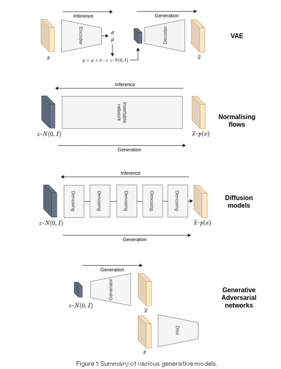
<p>Before we dive into diffusion models, let’s summarise the main methods for generating from a distribution currently available to us, and see how diffusion models look compared to them. This is shown in Figure 1.</p>

<p><img src="/images/diffusion_figure_1.png" alt="Figure 1: Summary of various generative models" /></p>

<h2 id="the-forward-process">The forward process</h2>

<p>The forward step in a diffusion model consists of adding small amounts of Gaussian noise to our image (which is sampled from our data distribution), until it looks like a Gaussian sample from \(N(0, I)\). We define a number of steps we want to achieve this transition in, and at each step, we add noise with a variance we pre-set (we call this the variance schedule). Since each transition depend only on the present state, the forward process is Markovian and can be written as:</p>

\[q(x_t | x_{t-1}) = N\left(x_t; \sqrt{1-\beta_t}x_{t-1}, \beta_t I\right)\]

\[q(x_{1:T} | x_0) = \prod_{t=1}^T q(x_t | x_{t-1})\]

<p>Here, \(\beta_t\) is our variance at time step \(t\). As well as adding noise, we also scale down the previous sample by \(\sqrt{1-\beta_t}\) which is required if we are to bound the variance of \(x_t\) in the limited of a standard normal. This will be graphically shown later.</p>

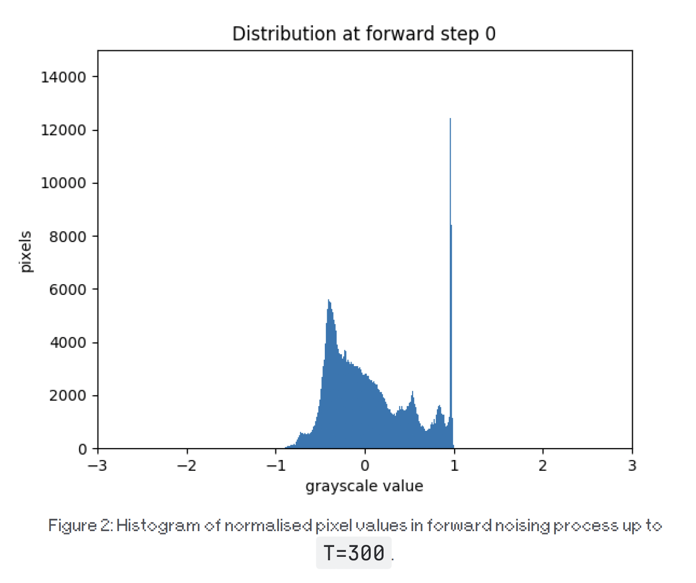
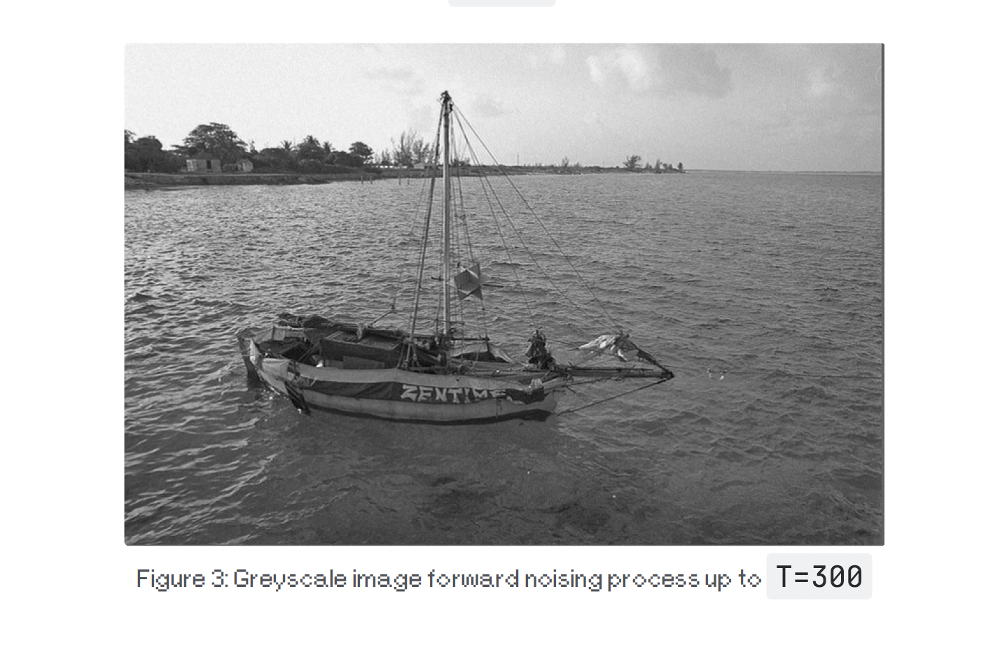
<p>Now, let’s see what this means in practice. Let’s take an image from the Kodak dataset, and define a variance schedule over \(T = 1000\) steps, starting at \(\beta = 10^{-4}\) and ending at \(\beta = 0.02\). Figures 2 and 3 below show a greay scale image and it’s grey value pixel distribution.</p>

<p><img src="/images/diffusion_figure_2.png" alt="Figure 2: Histogram of normalised pixel values in forward noising process up to T=300" /></p>

<p><img src="/images/diffusion_figure_3.png" alt="Figure 3: Greyscale image forward noising process up to T=300" /></p>

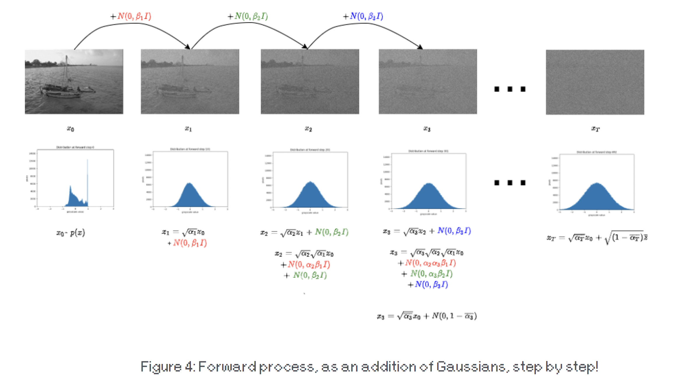
<p>Let’s have a closer look at what is actually happening in the forward noising process and some of its useful properties. Essentially, at each step \(t\) we are adding small amounts of Gaussian noise with a particular variance to the sample from the previous step, \(t-1\), while scaling it down with \(\sqrt{1-\beta_t}\). To help with notation, let’s write \(\beta_t = 1 - \alpha_t\). Figure 4 shows the forward step diagrammatically.</p>

<p><img src="/images/diffusion_figure_4.png" alt="Figure 4: Forward process, as an addition of Gaussians, step by step!" /></p>

<p>Figure 4 shows that at any point in the forward process, we can break down the current sample \(x_t\) into two terms:</p>

<ol>
  <li>
    <p>The initial data sample we are noising (\(x_0\) from \(p_x\)) and a cumulative product of scaling coefficients for \(x_0\), square root of \(\bar{\alpha}_t = \prod_{s=1}^t \alpha_s\) (which depends on the time step we are on and the self-defined variance schedule)</p>
  </li>
  <li>
    <p>A set of mean-zero Gaussian with different scales where the scales depend on the current time step and self-defined variance schedule. Using the properties of Gaussians, we can combine all these zero-mean Gaussians into one Gaussian with a particular variance, which is just the addition of the variance of all the Gaussians up to the point and takes the form \(1 - \bar{\alpha}_t\). A simple derivation of this is shown later.</p>
  </li>
</ol>

<h2 id="scaling-x">Scaling x</h2>

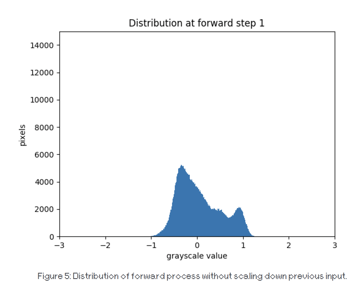
<p>Why do we need to scale down the previous input \(x_{t-1}\) at each step by the current variance? Well, let’s have a look at what happens if we don’t. Figure 5 shows the same process as Figure 4, but where the \(x_{t-1}\) is not scaled down by \(\sqrt{1-\beta_t}\). We observe that the variance of the distribution continues to grow and its tails become fatter, which means it is not an \(N(0, I)\).</p>

<p><img src="/images/diffusion_figure_5.png" alt="Figure 5: Distribution of forward process without scaling down previous input" /></p>

<h2 id="sampling-x_t-at-an-arbitrary-time-step-t">Sampling \(x_t\) at an arbitrary time step \(t\)</h2>

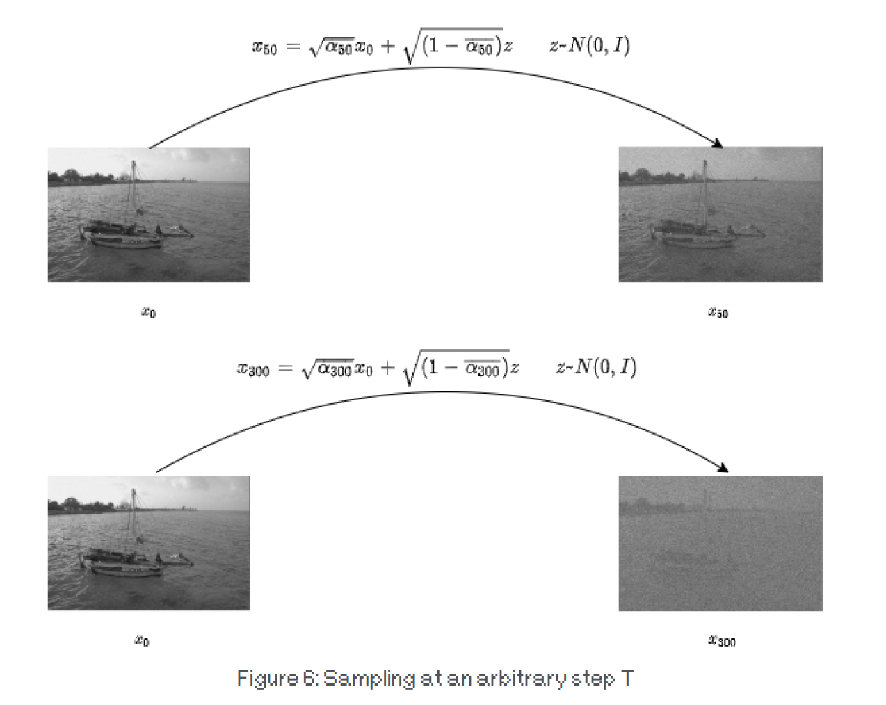
<p>Since we are adding a lot of Gaussians to a sample, this affords us the nice properties Gaussians bring with them. One useful property we can extract from this is the ability to sample a noisy \(x_t\) at any time step (without having to go through the entire forward process up to that point), given an \(x_0\). This is because we define the variance schedule and therefore, at any time steps, we know all the Gaussian samples that were added to \(x_0\) to get that particular noisy \(x_t\). Figure 4 already shows this, but here we provide more detail.</p>

\[t = 0:\]

\[x_0 \sim p_x(x)\]

\[t = 1:\]

\[x_1 = \sqrt{1-\beta_1}x_0 + N(0, \beta_1 I)\]

\[= \sqrt{1-\beta_1}x_0 + 0 + \sqrt{\beta_1}z_1\]

\[t = 2:\]

\[x_2 = \sqrt{1-\beta_2}x_1 + N(0, \beta_2 I)\]

\[= \sqrt{1-\beta_2}\left(\sqrt{1-\beta_1}x_0 + \sqrt{\beta_1}z_1\right) + \sqrt{\beta_2}z_2\]

\[= \sqrt{\alpha_2}\left(\sqrt{\alpha_1}x_0 + \sqrt{1-\alpha_1}z_1\right) + \sqrt{1-\alpha_2}z_2\]

\[= \sqrt{\alpha_2\alpha_1}x_0 + \sqrt{(1-\alpha_1)\alpha_2 + (1-\alpha_2)}\bar{z}\]

\[= \sqrt{\bar{\alpha}_2}x_0 + \sqrt{(1-\bar{\alpha}_2)}\bar{z}\]

<p><strong>For any \(t\):</strong></p>

\[x_t = \sqrt{\bar{\alpha}_t}x_0 + \sqrt{(1-\bar{\alpha}_t)}\bar{z}\]

<p>Here, \(z\) is a sample from a standard normal. The figure below demonstrates how we can jump from \(x_0\) directly to \(x_{50}\) and \(x_{100}\) though combining all the variances of the Gaussian in the chain up to those points. This is an extremely useful property and will help us in training as we shall see later.</p>

<p><img src="/images/diffusion_figure_6.png" alt="Figure 6: Sampling at an arbitrary step T" /></p>

<h2 id="the-reverse-process">The reverse process</h2>

<p>The true reverse process of our posterior is written as:</p>

\[p_\theta(x_{t-1} | x_t) = N(x_{t-1}; \mu_\theta(x_t, t), \Sigma_\theta(x_t, t)I).\]

<p>Like variational inference, we define an approximate distribution for our forward process \(q(x_{t-1} \mid x_t)\), and close the gap between the two using KL-divergence.</p>

<p>\(q(x_{t-1} \mid x_t)\) is generally intractable; however, it can be shown to be tractable when conditioned on \(x_0\). This results in the following formulation of what we call the forward process posterior:</p>

\[q(x_{t-1} | x_t, x_0) = \mathcal{N}\left( \mu_{\text{post}}, \tilde{\beta}_t I \right)\]

<p>where the posterior mean is:</p>

\[\mu_{\text{post}} = \frac{\sqrt{\bar{\alpha}_{t-1}}\beta_t}{1-\bar{\alpha}_t}x_0 + \frac{\sqrt{\alpha_t}(1-\bar{\alpha}_{t-1})}{1-\bar{\alpha}_t}x_t\]

\[\tilde{\beta}_t = \frac{\beta_t(1-\bar{\alpha}_{t-1})}{1-\bar{\alpha}_t}\]

<p>This can be derived with (2.116) in <a href="https://www.microsoft.com/en-us/research/uploads/prod/2006/01/Bishop-Pattern-Recognition-and-Machine-Learning-2006.pdf">Bishop’s book</a>. Therefore, if we can predict our posterior mean \(\mu_{\text{post}}\)
and our variance (which we can easily be computed as all terms are always known), we should be able to sample from our reverse posterior \(q(x_{t-1} | x_t, x_0)\).</p>

<p>If we have a look at this mean, during the reverse/sampling process, we know \(\bar{\alpha}\) and \(\beta\) as these are self-defined. \(x_t\) is the current step we are on, which we know too (since we start with a sample form \(N(0, I)\)). The only term we do not know at sampling time is \(x_0\). This is what we need a neural network to help us predict. We can train a network \(f_\theta(x_t, t)\) to directly predict this, given \(x_t\) and \(t\) as inputs, however, this is empirically shown not to work too well, and a better method is to do the following:</p>

<p>We know from the forward process that:</p>

\[x_t = \sqrt{\bar{\alpha}_t}x_0 + \sqrt{(1-\bar{\alpha}_t)}\varepsilon\]

<p>where \(\varepsilon \sim N(0, I)\) which we can rearrange to get an approximation of \(x_0\), say \(\tilde{x}_0\):</p>

\[\tilde{x}_0 = \frac{1}{\sqrt{\bar{\alpha}_t}}\left(x_t + \sqrt{1-\bar{\alpha}_t}\varepsilon\right)\]

<p>We can plug this formula in for \(x_0\) in the forward process posterior definition to obtain the reverse sampling step:</p>

\[x_{t-1} = \frac{1}{\sqrt{\alpha_t}}\left(x_t - \frac{\beta_t}{\sqrt{1-\alpha_t}}\varepsilon\right) + \tilde{\beta}_t z, \quad z \sim N(0, I)\]

<p>This leaves us with the unknown noise sample \(\varepsilon\) from a standard normal which we need to predict; all other terms are known. We can define a neural network to predict this term:</p>

\[\varepsilon \approx f_\theta(x_t, t) = \varepsilon_\theta\]

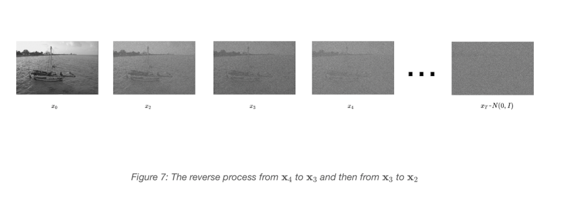
<p>Once we have estimated \(\varepsilon\), we can compute \(\tilde{x}_0\), after which we can predict \(\tilde{\mu}\) and sample the \(x_{t-1}\). Then we can repeat this process, until we get to \(x_0\) which is our sample from the distribution. Figure 7 shows this process in steps in the order they are performed during sampling, starting at \(x_4\) and predicting \(x_3\) and then \(x_2\).</p>

<p><img src="/images/diffusion_figure_7.png" alt="Figure 7: The reverse process from x_4 to x_3 and then from x_3 to x_2" /></p>

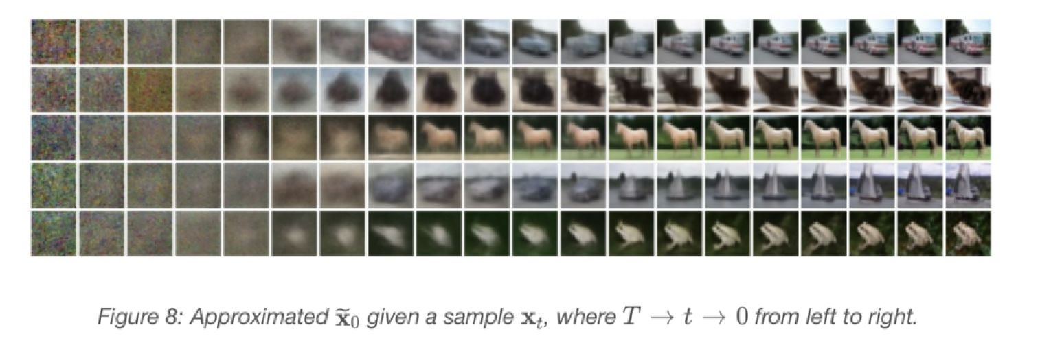
<p>What does \(\tilde{x}_0\) look like at each time step? That depends on where you are; if you are quite early in the chain, it looks like noise with some structure. If you are close to the end of the chain, it almost looks like an image. An example is shown in Figure 8, taken from the <a href="https://arxiv.org/abs/2006.11239">DDPM paper</a>.</p>

<p><img src="/images/diffusion_figure_8.png" alt="Figure 8: Approximated x̃_0 given a sample x_t, where T → t → 0 from left to right" /></p>

<h2 id="training">Training</h2>

<p>The loss function is a maximisation problem of the variational lower bound on the log-likelihood of the data:</p>

\[\mathbb{E}_q(x_0)[\log p_\theta(x_0)] \geq -\mathbb{E}_q(x_0)[\log q(x_{1:T} | x_0) - \log p_\theta(x_{0:T})] = -\mathcal{L}\]

<p>This can be reduced to a sum of KL-divergences between \(q(x_{t-1} \mid x_t, x_0)\) and \(p_\theta(x_{t-1} \mid x_t)\). Since both are Gaussian, this is just a KL between two Gaussians. Working through this, we can end up with a simplified loss term (we need to drop some scaling constants that arise when we do the KL between the Gaussians), corresponding to a weighted variational lower bound:</p>

\[\mathcal{L}_{\text{simple}} = \mathbb{E}_{x_0, \varepsilon}\left(\|\varepsilon - \varepsilon_\theta(x_t, t)\|_2^2\right)\]

<p>This is the simplified objective we can use to train our denoising function \(\varepsilon_\theta\), which is generally selected to be some sort of U-Net architecture. What this denoising function learns during training is the noise that was added to samples from the dataset to noise them. Once it is fully trained, it can then be used to remove that noise. The training process is then extremely simple and is performed as below:</p>

<ol>
  <li>
    <p>We select a random time step \(t\)</p>
  </li>
  <li>
    <p>We sample an instance of noise: \(\varepsilon \sim N(0, I)\)</p>
  </li>
  <li>
    <p>We generate the noisy sample \(x_t\) at this time step using the sampled noise \(\varepsilon\) and variance schedule (see forward process section)</p>
  </li>
  <li>
    <p>We feed this \(t\) and \(x_t\) to our denoising function \(\varepsilon_\theta(x_t, t)\) to approximate \(\varepsilon\)</p>
  </li>
  <li>
    <p>We use an L2-metric to compute a loss between \(\varepsilon\) and \(\varepsilon_\theta\)</p>
  </li>
</ol>

<h2 id="conditional-compression-denoising-decoder">Conditional compression denoising decoder</h2>

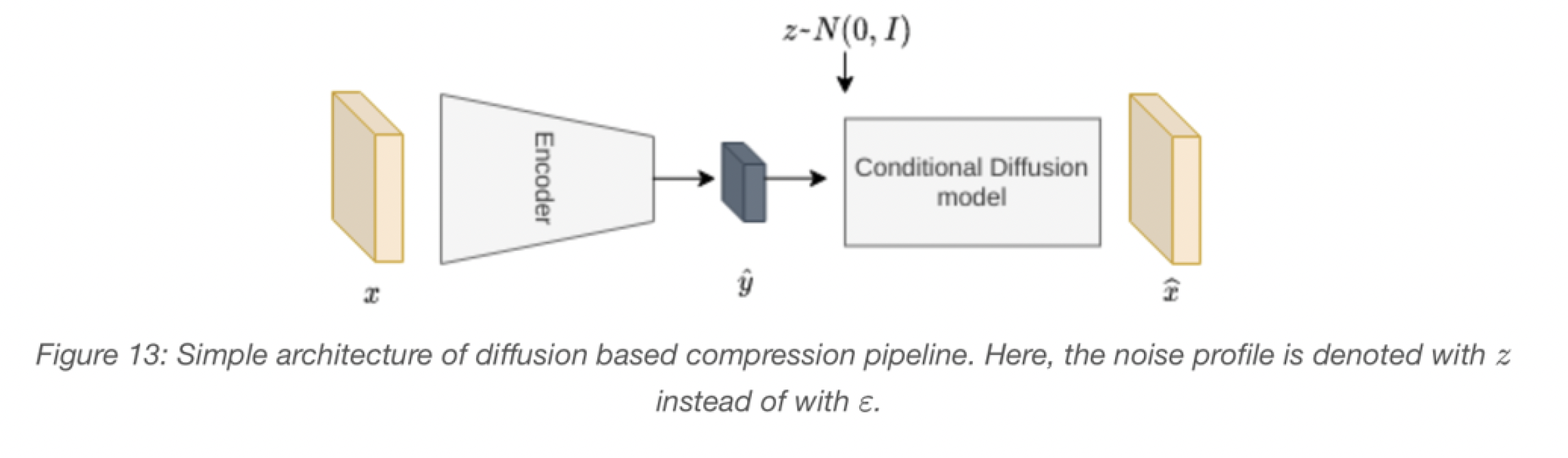
<p>Is there a way we could use diffusion models in our compression pipeline? Can they be used for explicit likelihood or implicit distribution matching?</p>

<p>An immediate idea would be to replace our decoder with a conditional diffusion model where we condition the diffusion process on the quantised latent space. This would enable conditional image generation allowing rate and distortion training as usual.</p>

<p>There are a few changes that we would need to consider for the pipeline. Let’s break them down into architecture, training and inference.</p>

<h3 id="architecture">Architecture:</h3>

<p>Until the decoder, our architecture can remain the same, however, we would then need to upsample our quantised latent space to the image scale (diffusion models work on the image scale).</p>

<p>We need to define a function \(\varepsilon_\theta\), which empirically is showed to work best as a U-Net architecture. The input of the U-Net will need to be a noise vector concatenated with an upsampled latent space.</p>

<h3 id="the-training">The training:</h3>

<p>The training function we minimise now becomes:</p>

\[L = \mathbb{E}_{x_0 \sim p(x_0)} \left( \mathbb{E}_{\varepsilon \sim N(0,I)} \left( \|\varepsilon - \varepsilon_\theta(x_t, t, \hat{y}_{us})\|_2^2 \right) + R \right)\]

<p>where \(\varepsilon\theta\) has an additional input to force it to be conditional.</p>

<h3 id="the-inference">The inference:</h3>

<p>The encoding works exactly the same, but the decoding differs. After the \(\hat{y}\) is produced, we sample a \(\varepsilon\), and perform the computation as shown in Figure 7 for some number of steps to get out final output \(\hat{x}\).</p>

<p><img src="/images/diffusion_figure_9.png" alt="Figure 9: Simple architecuture of a diffusion decoder based comprression pipeline. Here, the noise profile is denoted with $$eta$$, not $z$." /></p>

<p>I ran the above model and it produced competitive results on the first iteration. I have high hopes for the compression performance, but the largest concern is with execution time. We’d need to see a lot more algorithmic progress in diffusion decoders to enable efficient decoding.</p>]]></content><author><name>Arsalan Zafar</name><email>arsalanzafar@outlook.com</email></author><category term="AI based compression" /><category term="AI codecs" /><category term="Diffusion" /><summary type="html"><![CDATA[I’m always super interested in expanding the fronteir of learned compression. The current methods we use are derived from VAEs (equivalence shown here) and use GANs to improve preceptual quality but in this blog I explore how diffusion models could be used for compression.]]></summary></entry><entry><title type="html">Proof: MSE makes GANs locally stable</title><link href="https://arsalan-zafar.github.io/posts/2021/07/locally-stable-gans/" rel="alternate" type="text/html" title="Proof: MSE makes GANs locally stable" /><published>2021-07-21T00:00:00+00:00</published><updated>2021-07-21T00:00:00+00:00</updated><id>https://arsalan-zafar.github.io/posts/2021/07/Locally-Stable-GANs</id><content type="html" xml:base="https://arsalan-zafar.github.io/posts/2021/07/locally-stable-gans/"><![CDATA[<p>Generative Adversarial Networks are notoriously unstable due to issues such as mode collapse and training divergence. However, in AI compression, the adversarial training is generally stable and reliable without the neccessary tricks such as gradient penalty and adding noise to our input samples. I found this intriguing so I set out to explore why.</p>

<p>One obvious difference is that in compression GANs, we always have access to the ground truth image that we aim to generate. That allows us to use pixel-wise distortion losses in generator (encoder-decoder) training.</p>

<h2 id="convergence-of-gans">Convergence of GANs</h2>

<p>Our starting point is the <a href="https://arxiv.org/abs/1705.10461">Mescheder et al., 2017</a> Numerics of GANs paper. We can think of GAN training as a two-player non-cooperative game. The first player is a generator \(G_\theta(z)\) with parameters \(\theta\) that wants to maximize its payoff \(g(\theta, \psi)\), the second player is a discriminator \(D_\psi(x)\), with parameters \(\psi\) that aims to maximize \(d(\theta, \psi)\). The game is at a Nash equilibrium at \((\theta^*, \psi^*)\) when neither player can improve its payoff by changing its parameters slightly. When GAN reaches a Nash equilibrium, we can say that it reached local convergence.</p>

<p>One method to train a GAN is to use a Simultaneous Gradient Descent, which can be thought of as a fixed point algorithm that applies an operator \(F(\theta, \psi)\) to the parameters of the generator and discriminator \((\theta, \psi)\) respectively:</p>

\[F(\theta, \psi) = (\theta, \psi) + hv(\theta, \psi),\]

<p>where \(h\) is a learning rate and \(v(\theta, \psi)\) is the Jacobian of \(L\), our gradient:</p>

\[v(\theta, \psi) = \begin{bmatrix} -\nabla_\theta L(\theta, \psi) \\ \nabla_\psi L(\theta, \psi) \end{bmatrix}\]

<p>Mescheder et al. demonstrate that the convergence near an equilibrium point \((\theta^*, \psi^*)\) can be assessed by looking at the spectrum of Jacobian of our update operator \(F_h'(\theta, \psi)\) at the point \((\theta^*, \psi^*)\):</p>

<p>• If all eigenvalues have absolute value <strong>less than 1</strong>, the system <strong>converges to</strong> \((\theta^*, \psi^*)\) with a linear rate (our desired case).</p>

<p>• If there are any eigenvalues with absolute values <strong>greater than 1</strong>, the system <strong>diverges</strong>.</p>

<p>• If all eigenvalues have an absolute value <strong>equal to 1</strong> (lie on the unit circle), it can be convergent, divergent or neither, but if it is convergent, it will generally converge with a sublinear rate.</p>

<p>Now let’s look at a toy example to examine the conditions of convergence of GANs and discuss how the AI commpression objective impacts convergence. We’ll use the Dirac-GAN for simplicity with the non-saturating and vanillar loss for our analysis.</p>

<h2 id="dirac-gan">Dirac-GAN</h2>

<p>The Dirac-GAN consists of a (univariate) generator distribution \(p_g = \delta_\theta\) and a linear discriminator \(D_\psi(x) = \psi x\). The true data distribution \(p_D\) is given by a Dirac-distribution concentrated at 0.</p>

<p>Under this formulation, both the discriminator and the generator has exactly one parameter. This simplicity allows us to easily plot the vector field for the GAN in a 2D space to assess convergence behaviour. For a great explanation of vector fields and convergence of GANs, check out this <a href="https://inference.vc/my-notes-on-the-gan-literature/">inFERENCe blog post</a>.</p>

<p>The non-saturated GAN generator loss is:</p>

\[\max_\theta L(\theta, \psi) = f(-\psi\theta)\]

<p>where \(f(t) = -\log(1 + e^{-t})\). The discriminator loss is:</p>

\[\max_\psi L(\theta, \psi) = f(\psi\theta) - const\]

<p>The gradient vector is then:</p>

\[v(\theta, \psi) = \begin{bmatrix} -\psi f'(-\psi\theta) \\ \theta f'(\psi\theta) \end{bmatrix}\]

<p>The system has a unique equilibrium point of the training objective, at point \((\theta, \psi) = (0, 0)\). Indeed, since \(f(0) = const\), \(L(\theta, 0) = L(0, \psi) = const\) for all \(\theta, \psi \in \mathbb{R}\). Therefore \((\theta^*, \psi^*) = (0, 0)\) is a Nash-equilibrium. Now, assuming that \(f'(0) \neq 0\) we have that \(v(\theta, \psi) = 0\) only if \(\theta = \psi = 0\).</p>

<p>Now we can analyse the convergence of the Dirac-GAN around the equilibrium point \((\theta^*, \psi^*) = (0, 0)\) by calculating the Jacobian of the gradient vector field at the equilibrium point:</p>

\[v'(\theta, \psi) = \begin{bmatrix} f''(-\theta\psi)\psi^2 &amp; -f'(-\theta\psi) + f''(-\theta\psi)\theta\psi \\ f'(\theta\psi) + f''(\theta\psi)\theta\psi &amp; f''(\theta\psi)\theta^2 \end{bmatrix}\]

\[v'(0, 0) = \begin{bmatrix} 0 &amp; -f'(0) \\ f'(0) &amp; 0 \end{bmatrix}\]

<p>which has two eigenvalues, \(\pm f'(0)i\), which are both on the imaginary axis. This means that the model is not convergent with a linear rate, as it has zero real parts and we expect to see a circular vector field.</p>

<h2 id="adding-mse">Adding MSE</h2>

<p>Now, let us look at what happens by adding MSE to the loss for the generator parameters \(\theta\). The discriminator loss stays the same, but the generator loss becomes:</p>

\[\max_\theta L(\theta, \psi) = f(-\psi\theta) - (0 - \theta)^2\]

<p>The gradient vector field now has an additional \(-2\theta\) term is the \(\theta\) partial derivative:</p>

\[v(\theta, \psi) = \begin{bmatrix} -\psi f'(-\psi\theta) - 2\theta \\ \theta f'(-\psi\theta) \end{bmatrix}\]

<p>The Jacobian of the vector field becomes:</p>

\[v'(0, 0) = \begin{bmatrix} -2 &amp; -f'(0) \\ f'(0) &amp; 0 \end{bmatrix}\]

<p>And eigenvalues of the Jacobian of the gradient vector field at the equilibrium point is \(-1 \pm \sqrt{1 - f'(0)}\), both of which have negative real parts and 0 imaginary parts, which means that the system should be locally convergent around \((0, 0)\). The lack of imaginary parts means that there should not be any circular non-convergent behaviour in the gradient vector field.</p>

<h2 id="vanilla-gan-loss">Vanilla GAN loss</h2>

<p>We can repeat the analysis for the vanilla GAN loss function. The gradient vector is then:</p>

\[v(\theta, \psi) = \begin{bmatrix} -\psi f'(\psi\theta) \\ \theta f'(\psi\theta) \end{bmatrix}\]

<p>As before, the system has a unique equilibrium point of the training objective at the point \((\theta^*, \psi^*) = (0, 0)\).</p>

<p>The Jacobian of the gradient vector field at the equilibrium point:</p>

\[v'(\theta, \psi) = \begin{bmatrix} -f''(\theta\psi)\psi^2 &amp; -f'(\theta\psi) - f''(\theta\psi)\theta\psi \\ f'(\theta\psi) + f''(\theta\psi)\theta\psi &amp; f''(\theta\psi)\theta^2 \end{bmatrix}\]

\[v'(0, 0) = \begin{bmatrix} 0 &amp; -f'(0) \\ f'(0) &amp; 0 \end{bmatrix}\]

<p>which has two eigenvalues, \(\pm f'(0)i\), which are both on the imaginary axis. This means that the model is not convergent as it has zero real parts and we expect to see a circular vector field. Figure 4 demonstrates that Dirac-GAN with vanilla GAN loss is divergent around the equilibrium \((0, 0)\).</p>

<p>However, for similar reasons as above, the behaviour completely changes once we add the MSE component to the generator loss. The gradient vector field now has an additional \(-2\theta\) term in the \(\theta\) partial derivative:</p>

\[v(\theta, \psi) = \begin{bmatrix} -\psi f'(\psi\theta) - 2\theta \\ \theta f'(\psi\theta) \end{bmatrix}\]

<p>The Jacobian of the vector field becomes:</p>

\[v'(0, 0) = \begin{bmatrix} -2 &amp; -f'(0) \\ f'(0) &amp; 0 \end{bmatrix}\]

<p>And, just like in the case of non-saturating loss, eigenvalues of the Jacobian of the gradient vector field at the equilibrium point are \(-1 \pm \sqrt{1 - f'(0)}\).</p>

<p>This analysis shows that adding MSE has the same impact as gradient regularisation and instance noise, which also remove the circular behaviours in the gradient field and force the negative real part in the eigenvalues. This analysis explains how GANs in compresison can sidestep the need for these regaularization methods buy simple using the MSE.</p>

<h2 id="further-reading">Further reading:</h2>

<ul>
  <li>[1] Mescheder, Lars, Andreas Geiger, and Sebastian Nowozin. “Which training methods for GANs do actually converge?.” International conference on machine learning. PMLR, 2018. https://arxiv.org/pdf/1801.04406.pdf</li>
  <li>[2] Mescheder, Lars, Sebastian Nowozin, and Andreas Geiger. “The numerics of gans.” arXiv preprint arXiv:1705.10461 (2017). https://arxiv.org/pdf/1705.10461.pdf</li>
  <li>[3] Huszár Ferenc “GANs are Broken in More than One Way: The Numerics of GANs.” GANs are Broken in More than One Way: The Numerics of GANs. https://www.inference.vc/my-notes-on-the-numerics-of-gans/</li>
  <li>[4] Bertsekas, Dimitri P. “Nonlinear programming.” (1999). https://nms.kcl.ac.uk/osvaldo.simeone/bert.pdf</li>
  <li>[5] Theisel, Holger, and Tino Weinkauf. “Vector field metrics based on distance measures of first order critical points.” (2002). http://wscg.zcu.cz/wscg2002/Papers_2002/D49.pdf</li>
</ul>]]></content><author><name>Arsalan Zafar</name><email>arsalanzafar@outlook.com</email></author><category term="GANs" /><category term="Generative Adversarial Networks" /><category term="Machine Learning" /><category term="Deep Learning" /><category term="Pixel-wise losses" /><category term="Generative Compression Networks" /><summary type="html"><![CDATA[Generative Adversarial Networks are notoriously unstable due to issues such as mode collapse and training divergence. However, in AI compression, the adversarial training is generally stable and reliable without the neccessary tricks such as gradient penalty and adding noise to our input samples. I found this intriguing so I set out to explore why.]]></summary></entry><entry><title type="html">Cross-Entropy, KL and NLL are the same objective in AI compression</title><link href="https://arsalan-zafar.github.io/posts/2020/05/cross-entropy-kl-nll-ai-compression/" rel="alternate" type="text/html" title="Cross-Entropy, KL and NLL are the same objective in AI compression" /><published>2019-05-19T00:00:00+00:00</published><updated>2019-05-19T00:00:00+00:00</updated><id>https://arsalan-zafar.github.io/posts/2020/05/Cross-Entropy-KL-NLL-in-AI-Compression</id><content type="html" xml:base="https://arsalan-zafar.github.io/posts/2020/05/cross-entropy-kl-nll-ai-compression/"><![CDATA[<p>In end-to-end learned compression, we need to model the distribution of data, so we can entropy encode it. The training loss we use is the cross-entropy between the unknown true data distribution and our model distribution which in a simplest case is a fully factorized distribution of standard normals. There is often some confusion about the objective used in compression so I thought I’d use this post to clarify it. I’ll show that for data sampled from the true distribution \(p\) and a parametric model \(q_\theta\) we learn, the cross-entropy, the Kullback–Leibler divergence and the negative log-likelihood are optimization-equivalent objectives. In practice this means we are doing maximum likelihood estimation (MLE) and simultaneously minimizing expected code length.</p>

<h2 id="setup">Setup</h2>

<ul>
  <li>We assume samples \(x \sim p\) (the real data distribution).</li>
  <li>We train a model \(q_\theta(x)\) (density or probability mass) used for entropy coding and for likelihood.</li>
  <li>Expectations are with respect to \(p\): \(\mathbb{E}_p[\cdot] = \mathbb{E}_{x\sim p}[\cdot]\).</li>
</ul>

<h2 id="definitions-in-nats">Definitions (in nats)</h2>

<ul>
  <li>Cross-entropy of \(p\) under \(q_\theta\):</li>
</ul>

\[H(p, q_\theta) := \mathbb{E}_p\big[-\log q_\theta(x)\big].\]

<ul>
  <li>Shannon entropy of (p):</li>
</ul>

\[H(p) := \mathbb{E}_p\big[-\log p(x)\big].\]

<ul>
  <li>KL divergence (forward KL):</li>
</ul>

\[D_{\mathrm{KL}}(p\,\|\,q_\theta) := \mathbb{E}_p\big[\log p(x) - \log q_\theta(x)\big].\]

<ul>
  <li>Negative log-likelihood (NLL):</li>
</ul>

\[\mathrm{NLL}(\theta) := \mathbb{E}_p\big[-\log q_\theta(x)\big].\]

<h2 id="identities-and-immediate-consequences">Identities and immediate consequences</h2>

<p>By simple algebra,</p>

\[\begin{aligned}
H(p, q_\theta)
&amp;= \mathbb{E}_p\big[-\log q_\theta(x)\big]\\
&amp;= \mathbb{E}_p\big[\log p(x) - \log q_\theta(x)\big] + \mathbb{E}_p\big[-\log p(x)\big]\\
&amp;= D_{\mathrm{KL}}(p\,\|\,q_\theta) + H(p).
\end{aligned}\]

<p>Therefore</p>

\[H(p, q_\theta) \equiv \mathrm{NLL}(\theta) = D_{\mathrm{KL}}(p\,\|\,q_\theta) + H(p).\]

<p>Since \(H(p)\) does not depend on \(\theta\), the three quantities are <strong>minimization-equivalent</strong> in \(\theta\):</p>

\[\arg\min_\theta H(p, q_\theta) \;=\; \arg\min_\theta D_{\mathrm{KL}}(p\,\|\,q_\theta) \;=\; \arg\min_\theta \mathrm{NLL}(\theta).\]

<p>Equivalently,</p>

\[\arg\max_\theta \mathbb{E}_p\big[\log q_\theta(x)\big]\]

<p>which is the <strong>maximum likelihood estimator</strong> in expectation.</p>

<p>The latent space we model has dependencies, so a fully factorized mean-field approximation is too simple and will result in a large KL divergence. To improve modeling the joint distribution of our latents we need to compress, we can use a hyperprior model which introduces a latent that captures the dependencies and allows us to assume a fully factorized model, or we can break down our joint into a product of conditionals and use PixelCNN-like autoregressive models. Using conditional models (e.g., autoregressive context, hyperprior latents) preserves all identities by replacing \(q_\theta(x)\) with \(q_\theta(x\mid y)\) and taking expectations over the joint \(p(x,y)\).</p>

<h2 id="takeaways">Takeaways</h2>

<ul>
  <li>Training with cross-entropy loss in AI compression is the same as minimizing forward KL from the data distribution to the model and the same as minimizing population NLL.</li>
  <li>Consequently, we are performing MLE (maximizing \(\mathbb{E}_p[\log q_\theta(x)]\)).</li>
  <li>Minimizing this loss also minimizes the expected code length produced by an ideal entropy coder fed with \(q_\theta\).</li>
</ul>]]></content><author><name>Arsalan Zafar</name><email>arsalanzafar@outlook.com</email></author><category term="AI based compression" /><category term="Information Theory" /><category term="Likelihood" /><category term="Entropy coding" /><summary type="html"><![CDATA[In end-to-end learned compression, we need to model the distribution of data, so we can entropy encode it. The training loss we use is the cross-entropy between the unknown true data distribution and our model distribution which in a simplest case is a fully factorized distribution of standard normals. There is often some confusion about the objective used in compression so I thought I’d use this post to clarify it. I’ll show that for data sampled from the true distribution \(p\) and a parametric model \(q_\theta\) we learn, the cross-entropy, the Kullback–Leibler divergence and the negative log-likelihood are optimization-equivalent objectives. In practice this means we are doing maximum likelihood estimation (MLE) and simultaneously minimizing expected code length.]]></summary></entry></feed>